Accumulation
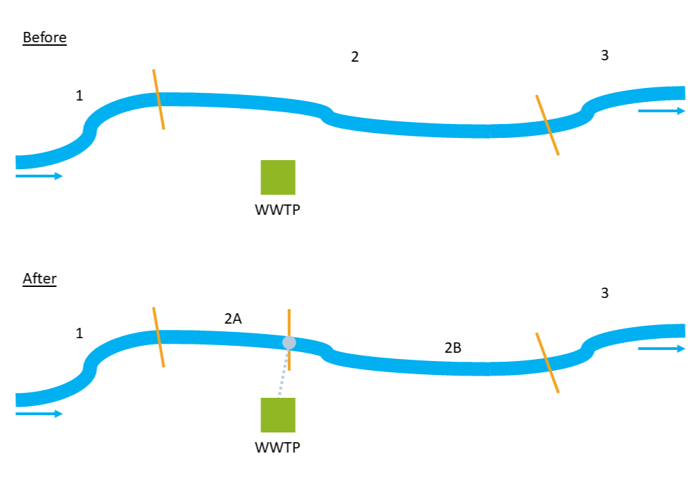
Fig. 7 How the division in extra river sections at WWTPs works within the plugin.
Once all WWTP emission points have been processed this way, API loads are progressively accumulated downstream along the network. Based on these accumulated loads and the flow values stored in the river shapefile, API concentrations are then calculated for each river section with formula (3). Two values are derived: concentration under mean flow conditions and concentration under mean low flow conditions.
With:
\(PEC\) = Predicted Environmental Concentration [\(ng/L\)]
\((m_{WW,eff})_{up}\) = load from all the upstream river section [\(kg/a\)]
\(Q\) = mean flow or mean low flow [\(m^3\!/s\)]
\(k\) = conversion factor [\(\frac{ng/kg \cdot m^3\!/L}{s/a}\)]
If WWTP annual effluent was added by the user in Emission Loads, a shapefile can be produced containing the dilution ratio calculated for each river section according to formula (4).
With:
\(DR\) = Dilution Ratio [\(-\)]
\(Q_{riv}\) = flow rate of river section [\(m^3\!/a\)]
\(Q_{WWTP,eff}\) = flow rate of WWTP effluent [\(m^3\!/a\)]
Additionally, if the user would like to calculate the modelled concentration at sampling campaign locations, it is possible to do so by providing to the tool a point shapefile. Thanks to this output, it will be easy to compare monitored vs modelled values and evaluate the performances of the model.
Input data
The following input data are required for this tool:
emission_loads.shp (from Emission Loads)
river_level.shp (from Flow Estimation)
monitoring_stations.shp [optional]
In case the user already has regionalized flow data, going through the Hydro-Module set of tools is not necessary. The important fields that should be in river_level.shp are:
ID field: a column with a unique ID for each river section
Next field: a column with the ID of the downstream river section
Accumulated mean flow: sum of the upstream mean flow values [\(m^3\!/s\)]
Accumulated mean low flow: sum of the upstream mean low flow values [\(m^3\!/s\)]
Regarding emission_loads.shp, the emission point should be at maximum 500 m from the closest river section, as stated before. If not, edit the location of the point. Same regarding monitoring_stations.shp.
Workflow
Add the input data to the project by clicking on “Layer -> Add Layer -> Add Vector Layer”
Go in the Processing Toolbox and look for the APRIORA plugin. Click on API emission and open 7 - Accumulation
Choose emission_loads.shp as input for API load
Select the fields containing the APIs to accumulate. This selection should include only columns containing load of APIs in kg/a.
Choose river_level.shp as input for River network
- Select the correct field of river_level.shp for ID Field, Next Field, Mean Flow, Acc. Mean Flow, Mean Low Flow and Acc. Mean Low Flow. In case river_level.shp is the output of Flow Estimation, here are the correct fields to select:
ID Field -> NET_ID
Next Field -> NET_TO
Acc. Mean Flow -> acc_Mean
Acc. Mean Low Flow -> acc_M_Low
Optional: 7. Choose monitoring_stations.shp as input for Monitoring Point 8. Click on the three dots positioned in the right of Monitoring station with modelled values and select a saving option 9. Repeat step 8 for Dilution Ratio 10. Click on Run
Output data:
river_accumulation.shp
monitoring_stations_with_modelled_values.shp [optional]
dilution_ratio.shp [optional]
The output river_accumulation.shp is a line shapefile containing the updated geometry of the river network. Its attribute table contains, for each section, the emitted load, the accumulated load and the resulting concentrations under both normal and low-flow condition for each API. Table 6 shows only a part of the attribute table for one substance and a few river sections.
NET_ID |
NET_TO |
Carb[kg/a] |
acc_Carb [1] |
conc_Carb [2] |
conL_Carb [3] |
|---|---|---|---|---|---|
1005 |
1006 |
0 |
17.789 |
39.422 |
150.251 |
1006 |
1007 |
0 |
17.789 |
39.265 |
149.398 |
1007 |
1008A |
0 |
17.789 |
39.134 |
148.712 |
1008A |
1008B |
0 |
17.789 |
38.615 |
148.277 |
1008B |
1009 |
3.68 |
21.469 |
41.873 |
168.519 |
1009 |
1010 |
0 |
21.469 |
41.671 |
167.611 |
1010 |
1011 |
0 |
21.469 |
41.368 |
166.652 |
1011 |
1012 |
0 |
21.469 |
40.693 |
164.549 |
The output monitoring_stations_with_modelled_values.shp is a point shapefile with the same geometry of monitoring_stations.shp and its attribute table is very similar to what is shown in Table 6.
The output of dilution_ratio.shp is a point shapefile with the same geometry of emission_loads.shp and its attribute table contains two extra columns, Q_Riv and Dilu_Ratio, which are respectively the flow rate of receving river section before its conversion in [\(m^3\!/a\)] and the dilution ratio.